
M1.D2: Introduction to Quantum Mechanics. Particle in a box.#
Learning Objectives#
Use the expression of the energy of a particle to investigate how the energy levels change by changing a) the mass of the particle, b) the length of the box, c) both the mass and the length.
Quantify the zero-point energy of the system and identify what variables affect its value.
Use magnitudes such as energy gaps and zero-point energy to quantify and compare the quantum vs classical behavior of two systems.
Plot the wavefunctions of a particle in a one-dimensional box for different particle masses and different box lengths. Plot the square of the wavefunctions and interpret it as density of probability to find the particle.
Context and goals
We saw that Bohr’s hydrogen atom gives us the energy levels that can reproduce the emission spectra of hydrogen. However, this is not a predictible model as it is not giving us the mechanics (how the system moves) of the atom. In order to understand how the atomic system moves we need to introduce quantum mechanics.
Quantum mechanics is so different from the physics that you probably know, with so many new concepts, that we will have to start slowly with the simplest of the quantum systems: The particle in a box, it’s not an atom, but it will help us understand some concepts when we tackle the quantum atom.
We want to know the equations of motion of the atom of Hydrogen (one proton and one electron) which we know must be studied with Quantum Mechanics. Before we solve that problem we will tackle the simplest of the problems in quantum mechanics, a free particle that does not interact with anything else but it is constained inside a box.
By solving this simple system we will come up with some terms that are useful to keep in mind, such as.
Hamiltonian
Schrodinger equation
Eigenfunctions and wavefunctions
Eigenvalues and energy values
Quantum numbers
Probability and density
The quantum/classical limit
Degeneracy
What are the equations to solve?#
The equations of motion are the equations that allow us to predict the motion of a system as it evolves over time.
In Classical mechanics (the non-quantum one) there are three main formulations of such equations of motion: the newtonian, the lagrangian, and the hamiltonian.
The one that you already know is the newtonian.
and being force the derivative of the energy over position $\( F=-\frac{dE(x)}{dr}\)\( we have \)\( -\frac{dE(x)}{dx} = m\frac{d^{2}x}{dt^{2}}\)$
Which is a partial diferential equation which solutions would be x(t), that is a function that tell us the position (x) of particles that make up the system at any given time. In the case of a falling particle under constant gravity force the solution is a function x(t) that tell us where the particle is at any given time.
The Schrodinger equation for a particle in a box (1-dimension)#
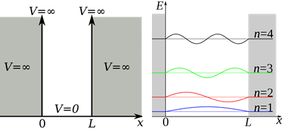
|

|
We won’t be spending much time on the algebra. However, there are some steps and some terms that need to be emphasized.
In quantum mechanics, the equations of motion are given by solving the Schrodinger equation.
$\( \hat{H}\Psi = E\Psi \)$
This is a partial partial differential equation. The solution to this equation is a function. In fact, this type of equation has as a solution a collection of functions. This collection of functions are called eigenfunctions
Think of it like a string in a guitar (see here https://en.wikipedia.org/wiki/Eigenfunction#Vibrating_strings). In how many ways can a string in a guitar vibrate? It can vibrate with the fundamental note, then the first overtone(octave), the second, the third.. and so on. The sine functions describing all the vibrations would be called eigenfunctions and the energy of the string would be their corresponding eigenvalue.
The wavefunction \(\Psi\) is an eigenfunction of the Schrodinger equation: it gives information about the position of the system
The Energy \(E\) is an eigenvalue of the Schrodinger equation: notice that the energy cannot have any value ,it is quantized (unlike a particle falling or any other classical system).
The “\(\hat{H}\)” is called the the Hamiltonian. And it has the form:
Where the variable “x” is the position. Because the particle in a box does not experience any potential inside the box, the overall Schrodinger equation to solve is
and their solutions are
Eigenfunctions (wavefunctions) : $\( \Psi(x)_n = \sqrt{\frac{2}{L}} sin\left(\frac{n \pi x}{L}\right) \)\( Eigenvalues (energies): \)\( E_n =\frac{h^2 n^2}{8 m L^2} \)$
Few things to observe
In the derivation of this equation one can see that the value of \(n\) can only have an integer positive number: \(n=1,2,3,4...\). Because of how the whole solution depends on the choice of \(n\), this number is called a quantum number
Notice that we have a collection of wavefunctions (eigenfunctions) that change depending on the value of “n”. If we change “n” the wavefunction changes.
The Schrodinger equation in this case is saying that if you derive twice the same function you should get the same function again multiplied by a parameter (eigenvalue) \(E\)
Let’s use the library “sympy” (if you don’t have it, install it using: conda install sympy, you’ll have to restart the Kernel)
If \(\Psi(x) = sin(\pi x)\) find the first and second derivative
from sympy import *

x, pi, n, L = symbols('x pi n L')
print("First derivative")
first = diff(sin(pi*x),x,1)
display(first)

print("Second derivative")
second=diff(sin(pi*x),x,2)
display(second)
First derivative
Second derivative
Can you trust a textbook? Try to derive twice what the textbook says it’s an eigenfunction of the Schdrodinger equation $\(\Psi(x) = \sqrt{\frac{2}{L}} sin\left(\frac{n \pi x}{L}\right)\)$
Use sympy to find $\(\frac{\delta \Psi(x)}{\delta x}\)\( and \)\(\frac{\delta^2 \Psi(x)}{\delta x^2}\)$
x, pi, n, L = symbols('x pi n L')
print("First derivative")
expr = sqrt(2/L)*sin(n*pi*x/L)
first = diff(expr,x,1)
display(first)
print("Second derivative")
second = diff(expr,x,2)
display(second)
First derivative
Second derivative
The quantized energy of the particle in a box#
Will energy levels be equally spaced?
Will they get closer at a higher quantum number “n”?
Will a higher mass affect the energy of the particle?
Will a larger box affect the energh of the particle?
h is Planck’s constant h = 6.626e-34 and m is the mass of the particle. In order to avoid very tiny numbers, we will use m=1 and h=1, so the Energy won’t be in Joules.
import matplotlib.pyplot as plt
import numpy as np
#Constants: we modify them so we can plot easy numbers. It's just a change of units (no Joules now!)
h = 1
m = 1


def getEnergyParticle(mass,n,length):
    return (h**2 * n**2)/(8*mass*length**2)

nmax = 10 #show the first ten levels of the particle in a box
L = 1
fig, ax = plt.subplots()

for n in range(1,nmax+1):
    ax.axhline(getEnergyParticle(m,n,L))
ax.set_xlabel("L")
ax.set_ylabel("Energy")
ax.set_title("Energy for box size L="+str(L)+" and mass="+str(m));

The effect of mass of the particle#
Let’s compare two boxes, one containing a mass double than the other. Before we plot them, think first about how the mass may effect the energy levels $\( E_n =\frac{h^2 n^2}{8 m L^2} \)$ remember is the quantum number and it can only be a positive integer n=1,2,3,4…
nmax = 10 #show the first ten levels of the particle in a box
L = 1

fig = plt.figure(figsize=(15,10))

ax1 = plt.subplot(121) #121 means: the subplots will be 1 row 2 columns and this one is subplot number 1
ax2 = plt.subplot(122, sharey = ax1) #share-y means that it will share the y-axis with the ax1 plot

thisMass = m
for n in range(1,nmax+1):
    ax1.axhline(getEnergyParticle(thisMass,n,L), 0, L, c='blue')
ax1.set_title("Energy levels for box size L="+str(L)+" and mass="+str(thisMass))
ax1.set_xlabel("L")
ax1.set_ylabel("Energy")
ax1.set_xlim(0,L)

thisMass = 2*m
for n in range(1,nmax+4+1):
    ax2.axhline(getEnergyParticle(thisMass,n,L), xmin=0, xmax=2, c='green')
ax2.set_title("Energy levels for box size L="+str(L)+" and mass="+str(thisMass))
ax2.set_xlabel("L")
ax2.set_xlim(0,L);

Effect of the size of the box#
Your turn. Compare two diagrams of the energy levels, one having the box size twice as long as the other.
Zero point energy#
Notice that the lowest Energy that a particle can have (n=1) it is not zero. This is residual energy that can never leave the system is called the Zero Point Energy and it is a very quantum (weird) property.
Also notice that the higher the mass, the lower this Zero Point Energy is. Again, the larger a system is the less quantum and more classical it behaves. (https://en.wikipedia.org/wiki/Zero-point_energy)
Calculate the Zero point energy for 4 cases. (Hint:there’s already a function defined above called getEnergyParticle)
m = 1, L = 1
m = 2, L = 1
m = 1, L = 2
m = 2, L = 2
The wavefunctions of the particle in a box and their meaning#
The wavefunction does not have as much physical meaning as its square. The square of the wavefunction \(\Psi^2(x)\) gives you the probability to find the particle.
Notice that the wavefunction does not depend on the mass
def psi(n,L,x):
    return np.sqrt(2/L)*np.sin(n*np.pi*x/L)
def psi_2(n,L,x):
    return np.square(psi(n,L,x))

#Values for L and x
L = 1
x_list = np.linspace(0,L,100) #this creates the numbers on the x axis
#choose a quantum number
n=1

#build the function
psi_2_list = []
psi_list = []
for x in x_list:
    psi_list.append(psi(n,L,x))
    psi_2_list.append(psi_2(n,L,x))
fig = plt.figure(figsize=(15,10))

ax1 = plt.subplot(121) #121 means: the subplots will be 1 row 2 columns and this one is subplot number 1
ax2 = plt.subplot(122, sharey = ax1) #share-y means that it will share the y-axis with the ax1 plot

ax1.plot(x_list, psi_list)
ax1.set_title("Particle in a box: Wavefunction L="+str(L)+" and n="+str(n))
ax1.set_xlabel("L")
ax1.set_ylabel("Ψ",fontsize=17)
ax1.set_xlim(0,L)

ax2.plot(x_list, psi_2_list)
ax2.set_title("Particle in a box: Wavefunction Squared L="+str(L)+" and n="+str(n))
ax2.set_ylabel("Ψ^2",fontsize=17)
ax2.set_xlabel("L")
ax2.set_xlim(0,L);

What should be the value of the integral of the wavefunction squared? Think about what should be the total probability if add up all the probabilities.
x, pi, n, L = symbols('x pi n L')
print("integration")

expr = (sqrt(2/L)*sin(n*pi*x/L))**2
display(expr)
result = integrate(expr, (x,0,L))
display(result)
integration
maxEigen = 5
L = 1
plt.figure(figsize=(15,10))
for n in range(1,maxEigen+1):
    #Empty lists for energy and psi wave
    psi_2_list = []
    psi_list = []
    for x in x_list:
        psi_2_list.append(psi_2(n,L,x))
        psi_list.append(psi(n,L,x))
    plt.subplot(maxEigen,2,2*n-1)
    plt.plot(x_list, psi_list)
    plt.xlabel("L", fontsize=13)
    plt.ylabel("Ψ", fontsize=13)
    plt.xticks(np.arange(0, 1, step=0.5))
    plt.title("Quantum number n="+str(n))
    plt.grid()
    plt.subplot(maxEigen,2,2*n)
    plt.plot(x_list, psi_2_list)
    plt.xlabel("L", fontsize=13)
    plt.ylabel("Ψ*Ψ", fontsize=13)
    plt.xticks(np.arange(0, 1, step=0.5))
    plt.title("Quantum number n="+str(n))
    plt.grid()

#conda install -c conda-forge ipywidgets
from ipywidgets.widgets import interact, Layout
Emax = 5
xmin = -2
Lmax = 5
def psi(n, x, L):
    return np.sqrt(2/L) * np.sin(n * np.pi * x / L)
def plt_psi(L):
    x = np.linspace(0,L,100)
    nmax = int(np.sqrt(Emax)*L)
    for n in range(1,nmax+1):
        plt.plot(x, psi(n,x,L)+(n/L)**2, c='r', lw=2, alpha=0.7)
        plt.axhline((n/L)**2, 0, L, c='k')
    plt.ylim(0,6)
    plt.xlim(xmin,Lmax+1)
    plt.axvspan(L, Lmax+1, fc='gray')
    plt.axvspan(-Lmax, 0, fc='gray')
    plt.show()
#to get this running you need to "trust this notebook" and reload page
interact(plt_psi, L=(1, Lmax, 0.1));
Notice that as we increase the size of the box (increasing L) the energy levels get closer and closer. To the point that there would be a continuum of energy, that is, the particle could have any energy and therefore the quantum nature will be lost. The take home message is that the quantum nature of systems disappears and becomes our familiar classical world as the systems (in this case the box) gets bigger.
Particle in a box in 2D#
If instead of just one dimension (x) we solve the Schrodinger equation in two dimensions (x and y), the wavefunctions have the following form
Notice that now there are two quantum numbers n and m and the box has two sides of length \(L_x\) and \(L_y\)
The energy also depends on the two dimensions. If you compare it to the energy in one dimension notice that it looks like the total energy is the sum of the energy on each dimension
An important concept here is degeneracy which is when more than one level has the same energy.
Degeneracy#
If we plot the different levels of the 2D particle in a box, we see that some levels have the same energy. For example, when the state (n=1,m=2) has the same energy as the state (n=2,m=1). We call these two states a degenerate state.
#build a energy level graph for particle in a box
h =1
def getEnergyParticle2d(mass,nx,ny,Lx,Ly):
    return (h**2)/(8*mass)*( (nx**2)/(Lx**2) + (ny**2)/(Ly**2))

fig = plt.figure(figsize=(15,10))
ax = plt.subplot()
nmax = 5
Lx = 1
Ly = 1
m =1

for nx in range(1,nmax+1):
    for ny in range(1,nmax+1):
        y=getEnergyParticle2d(m,nx,ny,Lx,Ly)
        ax.hlines(y,xmin=0.2,xmax=0.8)
        if nx < ny:
            delta = 0.1
        else:
            delta = 0
        ax.text(1+delta, y, str(nx)+','+str(ny), ha='left', va='center')

ax.set_ylabel("Energy")
ax.set_title("Energy levels for the 2D box size Lx="+str(Lx)+",Ly="+str(Ly)+" and mass="+str(m));
plt.xlim(0,Lx*1.2);

Your turn: Is there degneracy if the size of the 2D box is not a perfect square? Change Lx and Ly in the function above and show it.
Plotting the 2D wavefunctions#
#source: http://kleimanteach.chem.ufl.edu:4000/02_particle_in_an_infinite_potential_box.html
import matplotlib as mpl
# Defining the wavefunction
def psi2D(x,y): return 2.0*np.sin(n*np.pi*x)*np.sin(m*np.pi*y)

# Here the users inputs the values of n and m
n = int(input("Let's look at the Wavefunction for a 2D box \nEnter the value for n = "))
m = int(input("Enter the value for m = "))

# Generating the wavefunction graph
x = np.linspace(0, 1, 100)
y = np.linspace(0, 1, 100)
X, Y = np.meshgrid(x, y)
fig, axes = plt.subplots(1, 1, figsize=(8,8))
axes.imshow(psi2D(X,Y), origin='lower', extent=[0.0, 1.0, 0.0, 1.0])
axes.set_title(r'Heat plot of $\sqrt{L_xL_y}\Psi_{n,m}(x,y)$ for $n='+str(n)+r'$ and $m='+str(m)+r'$')
axes.set_ylabel(r'$y/L_y$')
axes.set_xlabel(r'$x/L_x$')

# Plotting the colorbar for the density plots
fig = plt.figure(figsize=(10,3))
colbar = fig.add_axes([0.05, 0.80, 0.7, 0.10])
norm = mpl.colors.Normalize(vmin=-2.0, vmax=2.0)
mpl.colorbar.ColorbarBase(colbar, norm=norm, orientation='horizontal')

# Show the plots on the screen once the code reaches this point
plt.show()
For other displays of the 2D particle in a box you can check here: akey7/basic-quantum-models
Particle in a box in 3D#
Of course the particle in a box can be expanded to the three dimensions of space \(x,y,z\). In this case there are three independent quantum numbers \(n,m,l\)
and the wavefunctions are the sin product for the three dimensions
Plotting a 3D function means that we need a 4th dimension which makes it hard to visualize. This is why we need to come up with a cutoff or threshold that allows us to draw an isosurface where the function has that value.
#source: https://github.com/wmfschneider/CHE30324/blob/master/Outline/CHE30324-outline.org
# conda install -c plotly plotly
import plotly.graph_objects as go
import numpy as np

#It has now three quantum numbers. Change these to see what it looks like
l = 2
m = 2
n = 1

xmesh=[]
ymesh=[]
zmesh=[]
# psi=np.array([])
psi=[]
points=25

for z in np.linspace(0.,1.,points):
    for y in np.linspace(0.,1.,points):
        for x in np.linspace(0.,1.,points):
            xmesh.append(x)
            ymesh.append(y)
            zmesh.append(z)
            value=np.sin(l*np.pi*x)*np.sin(m*np.pi*y)*np.sin(n*np.pi*z)
            psi.append(value)
#            np.append(value,psi)
#            print("{0:8.6f} {1:8.6f} {2:8.6f} {3:8.6f}".format(x,y,z,value))

# print(zmesh)
#print(psi)
iso = 0.1

fig= go.Figure(data=go.Isosurface(
    x=xmesh,
    y=ymesh,
    z=zmesh,
    value=psi,
    isomin=-iso,
    isomax=iso,
    surface_count=2,
    opacity=0.5,
    caps=dict(x_show=False, y_show=False,z_show=False)
))

fig.show()
References#
For more information about what a hamiltonian is in classical physics see here

Questions#
Create a new notebook with proper headers, writing the questions
Are the energy levels equally spaced? Write the formula for the energy of the particle and explain what factors makes it not equally spaced? Plot the energy levels indicating what L and mass you have used.
What is the effect of making the mass of the particle larger? 2.1 Plot two adjacent plots for the particle in a box, both of length 5 units. Graph on the left with mass = 3 units and the graph on the right with mass = 4 Comment on the differences.
What is the effect of making the box larger? 3.1 Plot two adjacent plots for the particle in a box, both of mass 5 units. Graph on the left with length = 3 units and the graph on the right with length = 4. Comment on the differences.
Looking at the effect of length of the box and the mass of the particle. What will make the system less quantum-like, doubling the mass or doubling the size of the box?
What will have a larger zero point energy, a system with a larger mass or smaller mass? a system with a larger box size or smaller box size?
Calculate the Zero point energy for 4 cases m = 1, L = 1 m = 2, L = 1 m = 1, L = 2 m = 2, L = 2 do these results match with your answer on question 4?
Challenge: write a function that calculates the energy of the particle in a box for 3D given n, l, m and Lx, Ly, Lz.
Further challenge: write a table showing the energy for all the possible combinations of n,l,m where n,l,m can have any number from 1 to 4.